An output-only interface completeness metric based on generalized transmissibility

Authors

Affiliation

JWR Meggitt

Acoustics Research Centre, The University of Salford, UK

R McGee

Acoustics Research Centre, The University of Salford, UK

Abstract

Interface completeness is a key requirement for the successful representation of interface dynamics, as required by in-situ blocked force characterization and structural decoupling. To quantify interface completeness an FRF-based metric termed the ICC has been proposed and shown to correlate well with blocked force validations. The main limitation of the ICC is the need to complete an expensive FRF measurement campaign before being able to compute it; in particular the full interface FRF matrix is required. If the chosen representation is then insufficient, additional DoFs must be added and the ICC test repeated. Ideally, one would obtain a metric for the completeness of an interface using only operational measurements, reducing both time and uncertainty. In the present paper we investigate the use of generalized transmissibilities (GTs) to formulate a completeness metric using output-only measurements. By using the constraints present within the definition of GT, we are able to mathematically constrain an interface using only operational response. If complete, the GTs that traverse the interface should be zero. We use this fact to establish a Transmissibility-based ICC (TICC). Through numerical and experimental examples we show that the TICC correlates well with the standard ICC whilst providing a simpler and more robust experimental identification.

Keywords

Interface completeness, Generlized transmissibilities, Interface dynamics

1 Introduction

In component-based modelling and virtual prototyping, it is often said that everything goes right or wrong at the interface [1]. It is at the interface where we represent the active and passive dynamics of a component, and where we enforce continuity and equilibrium between coupled components. Key to the success of any characterisation method or assembly process is the complete representation of the interface dynamics; all significant DoFs at the interface must be captured by the chosen representation.

To minimize uncertainty and improve confidence in our modelling efforts, it is therefore beneficial to quantify, in some way, the completeness of an interface representation. Poor measures of completeness can be used to guide further refinement of the interface representation or identify frequency ranges that are more susceptible to errors. To this end, the Interface Completeness Crtierion (ICC) was proposed in [2]. The ICC has since been used in a number of studies to quantify interface completeness, and is available in commercial software for this purpose [3].

The ICC is based on the observation that if the interface representation is complete, then a transfer admittance that traverses the interface can be decomposed exactly into the product of three sub-matrices that together form a transmission path across the interface. The ICC quantifies the degree to which this decomposition holds, with a value of 1 indicating a complete interface, and \(<<1\) an incomplete interface. Whilst the ICC has shown good correlation with blocked force validations, it suffers from two notable limitations. First, it is necessary to perform a full set of interface FRF measurements to compute the ICC; this can be time consuming and prone to experimental error. Second, the ICC is based entirely on passive FRF measurements and so does not take into account which interface DoFs are significant whilst the assembly is active (for example in a blocked force characterisation). In the present paper, we propose an alternative completeness metric that avoids these limitations.

Based on the notion of generalised transmissibilities (GTs) [4], we propose the Transmissibility-based ICC (TICC). Fundamentally, is based on the blocking constraints present within the GT definition and yields an output similar to the conventional ICC; a value of 1 indicating a complete interface and a value \(<<1\) an incomplete one. Importantly, the TICC avoids the need to measure any interface FRFs and can be computed using conventional FRFs, output-only response measurements, or a combination thereof.

In this paper we present the mathematical formulation of the TICC, and illustrate its use through numerical and experimental examples. We compare the TICC against the conventional ICC and show that they are in good agreement. The results suggest that the TICC can be used as a more robust alternative to the ICC for quantifying interface completeness.

Having outlined the context of this paper, its remainder will be structured as follows. In Section 2 we introduce the notion of interface completeness, before presenting the established ICC, and the newly proposed TICC metric. In Section 3 we present a numerical example to illustrate the TICC, followed by an experimental example in Section 4. Finally, in Section 5 we draw some concluding remarks and outline some further studies.

2 Interface completeness

We introduce the notion of completeness by way of the in-situ blocked force method [5], though the concept is more general and applies to any method that requires an experimental representation of interface dynamics, e.g. structural coupling/decoupling.

The in-situ blocked force relation states that the operational response of an assembly at some receiver-side location \(r\) due to the internal operating forces of a source subsystem can be reconstructed by applying the (negative) blocked forces of the source subsystem at the coupled interface \(c\) with the receiver subsystem (we omit the negative sign here as practically it makes no difference), \[ \mathbf{v}_{r} = \mathbf{Y}_{Crc}\bar{\mathbf{f}}_c \tag{1}\] This relation is used inversely to estimate the blocked forces of the source subsystem from operational response measurements, typically made at (or close to) the interface (\(r\rightarrow c\)), \[ \bar{\mathbf{f}}_c = \mathbf{Y}_{Ccc}^{-1}\mathbf{v}_{c} \tag{2}\]

In practice, only a subset of all possible interface DoFs are measured and used to estimate the blocked forces. We denote the measured interface DoFs as \(c_i\) and the unmeasured interface DoFs as \(c_j\). The blocked force relation can then be partitioned as, \[ \mathbf{v}_{c_i} = \mathbf{Y}_{Cc_ic}\bar{\mathbf{f}}_c = \overbrace{\mathbf{Y}_{Cc_ic_i}\bar{\mathbf{f}}_{c_i}}^{\mathrm{Known \, DoFs}} + \overbrace{\mathbf{Y}_{Cc_ic_j}\bar{\mathbf{f}}_{c_j}}^{\mathrm{ Unknown \, DoFs}} \tag{3}\] Pre-multiplying Equation 3 by the inverse of \(\mathbf{Y}_{Cc_ic_i}\) allows us to estimate the blocked force \(\bar{\mathbf{f}}_{c_i}\), \[ \mathbf{Y}_{Cc_ic_i}^+\mathbf{v}_b = \underbrace{\bar{\mathbf{f}}_{c_i} + \overbrace{\mathbf{Y}_{Cc_ic_i}^+\mathbf{Y}_{Cc_ic_j}\bar{\mathbf{f}}_{c_j}}^{\mathrm{Bias \, error}}}_{\mathbf{\tilde{\bar{f}}}_{c_i}} \tag{4}\] However, we see that by neglecting the \(c_j\) DoFs, we have introduced an error onto the blocked force, resulting in the biased estimate \(\mathbf{\tilde{\bar{f}}}_{c_i}\).

The dynamics contained within the bias error are those of the initial assembly \(C\), meaning the estimated blocked force is no longer an intrinsic property of the source subsystem \(S\). Depending on the relative importance of the omitted DoFs \(c_j\), the bias error may be negligible (if the interface is sufficiently complete) or quite significant (if it is incomplete). In either case, this bias error will propagate through any future calculations involving the blocked force, and thus limit our predictive accuracy.

2.1 FRF-based completeness (ICC)

To minimize the bias error in Equation 4, we need to ensure that the chosen interface representation is sufficiently complete, i.e. that \(c_i\) contains all the DoFs that are important to describe the interface dynamics.

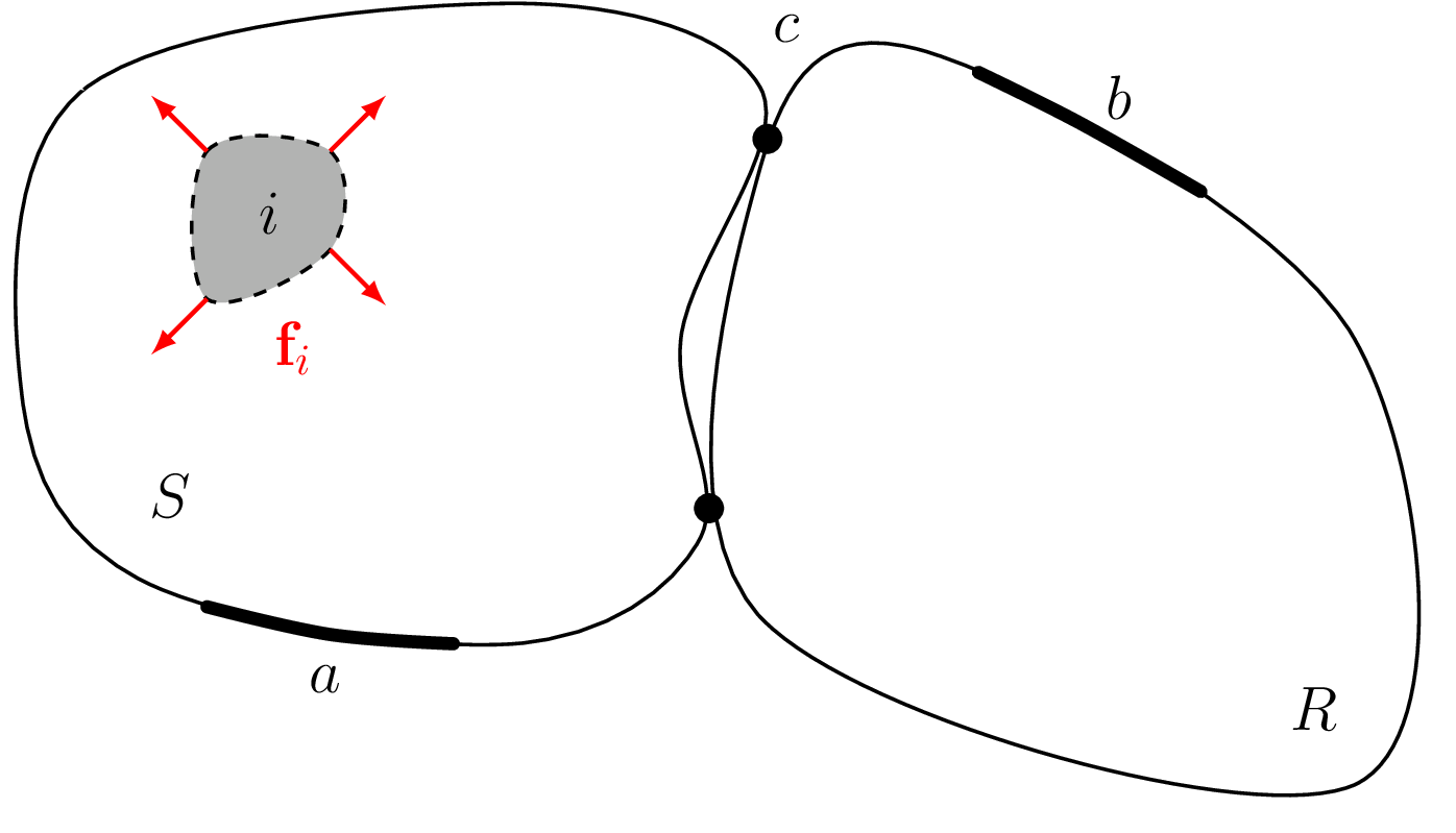
Figure 1: Coupled \(SR\) assembly with internal source DoFs \(i\), remote source DoFs \(a\), interface DoFs \(c\), and remote receiver DoFs \(b\).

In [2] the Interface Completeness Criterion (ICC) was proposed for this purpose. The ICC is based on the observation that if the interface representation is complete, then the transfer admittance between remote source DoFs \(a\) and remote receiver DoFs \(b\) should be fully captured by transmission paths that traverse the interface DoFs \(c\), and can be reconstructed exactly through [6] , \[ \mathbf{Y}_{Cba} = \mathbf{Y}_{Cbc}\mathbf{Y}_{Ccc}^{-1}\mathbf{Y}_{Cca} \tag{5}\]

In practice, the complete set of interface DoFs \(c\) is not available, and so we can only form an approximate reconstruction using the measured interface DoFs \(c_i\), \[ \mathbf{Y}_{Cba} \stackrel{?}{\approx} \mathbf{Y}_{Cba}^{(c_i)} = \mathbf{Y}_{Cbc_i}\mathbf{Y}_{Cc_ic_i}^{-1}\mathbf{Y}_{Cc_ia} \tag{6}\] Equation 6 can be interpreted as an onboard validation for an artificial blocked force; the FRF product \(\mathbf{Y}_{Ccc}^{-1}\mathbf{Y}_{Cca}\) yields a blocked force for each of the normalised responses in the columns of \(\mathbf{Y}_{Cca}\). Pre-multiplication by \(\mathbf{Y}_{Cbc}\) then uses these blocked forces to reconstruct the response at \(b\). The FRF \(\mathbf{Y}_{Cba}\) describes the directly response measured at \(b\) due to the same set of artificial forces at \(a\).

The ICC quantifies the degree to which this approximation holds, with a value of 1 indicating exact reconstruction (i.e. a complete interface) and a value \(<<1\) indicating poor reconstruction (i.e. an incomplete interface). The ICC is most commonly defined as, \[ \mathrm{ICC} = \mbox{Corr}\left(\vec{\mathbf{Y}}_{Cba}, \vec{\mathbf{Y}}_{Cba}^{(c_i)} \right) \] where \(\vec{\square}\) denotes matrix vectorisation and \(\mbox{Corr}(\square,\square)\) is a correlation-based measure of similarity (like the MAC [7]) between the two vector arguments. Other definitions of the ICC are possible, for example in [8] a coherence-style comparision is made between \(\mathbf{Y}_{Cba}\) and \(\mathbf{Y}_{Cba}^{(c_i)}\), and in [9] a combined correlation/coherence-based metric is used (termed ICC+).

Experimentally, the ICC is straightforward to compute however, it does require the measurement (and subsequent inversion) of the interface FRF matrix \(\mathbf{Y}_{Ccc}\). This is often a time consuming measurement and an error prone step which we would generally prefer to avoid if possible.

2.2 GT-based completeness (TICC)

To avoid the measurement effort associated with the ICC described above, we look to use generalised transmissibilities (GTs) to formulate an alternative completeness metric. The advantage of GTs is that they can be estimated using only output (response) measurements, without the need to apply any known forces.

The general definition of a (response-based) GT matrix \(\mathbf{T}_{ba}\) between two sets of DoFs, \(a\) and \(b\), is given by, \[ \left(\begin{array}{c} v_{b_1} \\ v_{b_2} \\ \vdots \\ v_{b_m} \end{array}\right) = \overbrace{\left[\begin{array}{c c c c} T_{b_1a_1} & T_{b_1a_2} & \cdots & T_{b_1a_n} \\ T_{b_2a_1} & T_{b_2a_2} & \cdots & T_{b_2a_n} \\ \vdots & \vdots & \ddots & \vdots \\ T_{b_ma_1} & T_{b_ma_2} & \cdots & T_{b_ma_n} \end{array}\right]}^{\mathbf{T}_{ba}} \left(\begin{array}{c} v_{a_1} \\ v_{a_2} \\ \vdots \\ v_{a_n} \end{array}\right) \quad \quad T_{b_ia_j} = \frac{v_{b_i}}{v_{a_j}}\Bigg|_{v_{a_k}=0\, \forall \, k\neq j} \] An important observation is that the element-wise definition of the GT elements \(T_{b_ia_j}\) involves rigidly constraining all DoFs \(k\neq j\) in set \(a\) to be zero.

The idea behind the TICC is to use this rigid constraint to block transmission across the interface. To achieve this, we consider the GT between a set of remote receiver DoFs \(b\) and the combined set of remote source (\(a\)) and interface (\(c\)) DoFs, \[ \mathbf{v}_b = \left[\begin{array}{cc} \mathbf{T}_{bc} & \mathbf{T}_{ba} \end{array} \right] \left(\begin{array}{c}\mathbf{v}_c \\ \mathbf{v}_a\end{array}\right) \] Considering the sub-GT matrix \(\mathbf{T}_{ba}\) (whose element-wise definition includes a constraint over the interface DoFs \(c\)), \[ \mathbf{v}_b = \mathbf{T}_{ba} \Big|_{\mathbf{v}_c = 0} \mathbf{v}_a = \mathbf{0} \, \mathrm{(if \, complete)} \] we reason that if the interface representation is complete, then constraining the interface DoFs \(c\) to zero should block all transmission paths between the remote source DoFs \(a\) and remote receiver DoFs \(b\), resulting in \(\mathbf{T}_{ba} = \mathbf{0}\). If the interface representation is incomplete, some transmission paths will remain unblocked, resulting in \(\mathbf{T}_{ba} \neq \mathbf{0}\). The TICC is based on an assessment of \(\mathbf{T}_{ba} \stackrel{?}{=} \mathbf{0}\).

For a more detailed proof that \(\mathbf{T}_{ba} = \mathbf{0}\) for a complete interface, we consider the equation of motions for the \(SR\) assembly depicted in Figure 1, \[ \left(\begin{array}{c} \mathbf{f}_i \\ \mathbf{0} \\ \mathbf{0} \end{array}\right) = \left[\begin{array}{c c c} \mathbf{Z}_{ii} & \mathbf{Z}_{ix} & \mathbf{0} \\ \mathbf{Z}_{xi} & \mathbf{Z}_{xx} & \mathbf{Z}_{xb} \\ \mathbf{0} & \mathbf{Z}_{bx} & \mathbf{Z}_{bb} \\ \end{array}\right]\left(\begin{array}{c} \mathbf{v}_i \\ \mathbf{v}_x \\ \mathbf{v}_b \end{array}\right) \tag{7}\] where we have grouped together the remote source and interface DoFs such that \(x = \{a \,, c\}\). Writing out the last line of Equation 7, \[ \mathbf{0} = \mathbf{Z}_{bx} \mathbf{v}_x + \mathbf{Z}_{bb}\mathbf{v}_b \] we rearrange to obtain the relation, \[ \mathbf{v}_b = \mathbf{Z}_{bb}^{-1}\mathbf{Z}_{bx} \mathbf{v}_x = \mathbf{T}_{bx} \mathbf{v}_x \] where \(\mathbf{T}_{bx}\) is the transmissibility between the combined \(x = \{a \,, c\}\) DoFs and the remote receiver DoFs \(b\), due to the internal operating force \(\mathbf{f}_i\). If we now separate the \(a\) and \(c\) DoFs, \[ \begin{aligned} \mathbf{v}_b &= \mathbf{Z}_{bb}^{-1} \left[\begin{array}{cc} {\color{red}\mathbf{Z}_{ba}} & \mathbf{Z}_{bc} \end{array}\right]\left(\begin{array}{c} \mathbf{v}_{a} \\ \mathbf{v}_{c} \end{array}\right)\\ &= \left[\begin{array}{cc} {\color{red}\mathbf{T}_{ba/x}} & \mathbf{T}_{bc/x} \end{array}\right] \left(\begin{array}{c} \mathbf{v}_{a} \\ \mathbf{v}_{c} \end{array}\right) \end{aligned} \] we obtain two sub-GT matrices, \(\mathbf{T}_{ba/x}\) and \(\mathbf{T}_{bc/x}\), where the subscript \(/x\) reminds us that the transmissibility as been defined in terms of the combined DoF set \(x\).

Noting that for a complete interface representation, the transfer impedance \(\mathbf{Z}_{ba}=\mathbf{0}\), we see that \(\mathbf{T}_{ba/x}=\mathbf{0}\) also, i.e. the interface has been completely blocked by the constraints imposed at \(c\). If some DoFs are omitted from the interface representation, some transmission paths will remain unblocked, and so \(\mathbf{T}_{ba}\neq\mathbf{0}\).

To determine the sub-GT matrix \(\mathbf{T}_{ba}\) from output-only measurements, we consider the operational response of the assembly in \(N_s\) independent states (e.g. operating speeds, load cases, etc.), resulting in the response matrices \(\mathbf{V}_a \in\mathbb{C}^{N_a\times N_s}\), \(\mathbf{V}_c\in\mathbb{C}^{N_c\times N_s}\) and \(\mathbf{V}_b\in\mathbb{C}^{N_b\times N_s}\), with each column representing an independent operational state. The GT relation can then be written in matrix form and solved using the matrix pseudo-inverse as, \[ \mathbf{V}_b = \left[\begin{array}{cc} \mathbf{T}_{ba} & \mathbf{T}_{bc} \end{array} \right] \left[\begin{array}{c}\mathbf{V}_a \\ \mathbf{V}_c\end{array} \right] \quad \rightarrow \quad \left[\begin{array}{cc} \mathbf{T}_{ba} & \mathbf{T}_{bc} \end{array} \right] = \mathbf{V}_b \left[\begin{array}{c}\mathbf{V}_a \\ \mathbf{V}_c\end{array} \right]^+ \] from which we can extract the sub-GT matrix \(\mathbf{T}_{ba}\).

Note that the columns of \(\mathbf{V}_a\), \(\mathbf{V}_b\) and \(\mathbf{V}_c\) need not be strictly operational responses; they could also be responses normalised to a known input force excitation, i.e. FRF measurements. Considering the normalised responses at \(b\), \(a\) and \(c\) due to a set of known forces at \(i\), we can write the GT as, \[ \left[\begin{array}{cc} \mathbf{T}_{ba} & \mathbf{T}_{bc} \end{array} \right] = \mathbf{Y}_{bi} \left[\begin{array}{c}\mathbf{Y}_{ai} \\ \mathbf{Y}_{ci}\end{array} \right]^+ \] In general, we can combine operational response measurements and FRFs compute a more robust GT.

Finally, to quantify the degree of completeness we need to determine the degree to which \(\mathbf{T}_{ba}\) deviates from zero. This can be done in a variety of ways. Here we define the TICC as, \[ \mathrm{TICC} = 1 - \frac{2||\mathbf{T}_{ba/x}||_F^2}{||\mathbf{T}_{ba/x}||_F^2 + ||\mathbf{T}_{ba}||_F^2} \tag{8}\] where \(||\cdot||_F\) is the Frobenius norm, \(\mathbf{T}_{ba/x}\) is the sub-GT obtained when including the interface DoFs \(c\) (thus constraining them), and \(\mathbf{T}_{ba}\) is the GT matrix obtained when excluding the interface DoFs (the interface is unconstrained).

Inspecting Equation 8, we see that a complete interface representation results in \(\mathbf{T}_{ba/x}=\mathbf{0}\), and so the TICC is 1. Regarding the lower bound, omitting the factor of 2 would provide a TICC bounded between 0 and 1, like the ICC. However, the factor of 2 is included to add some physically; if the interface is completely unconstrained, \(\mathbf{T}_{ba/x}=\mathbf{T}_{ba}\), resulting in a TICC of 0. Values less than zero indicate an amplification of transmission due to the constraints at \(c\).

Like the ICC, the TICC is bounded between 0 and 1, with a value of 1 indicating a complete interface representation. We believe the advantages of the TICC are three fold: 1) it can in principle be computed using output-only response measurements without the need to measured any FRFs; 2) it can alternatively be computed using FRFs only, whilst avoiding the need to excite the interface; and 3) it enables FRFs and operational responses to be used in combination to provide a more robust estimate of interface completeness.

3 Numerical example - continuous plate-plate system

In this section we present a numerical example to illustrate the proposed TICC. We consider a continuous simply-supported plate, similar to that used in [2], for which we compare the TICC against the FRF-based ICC for different levels of interface discretisation.

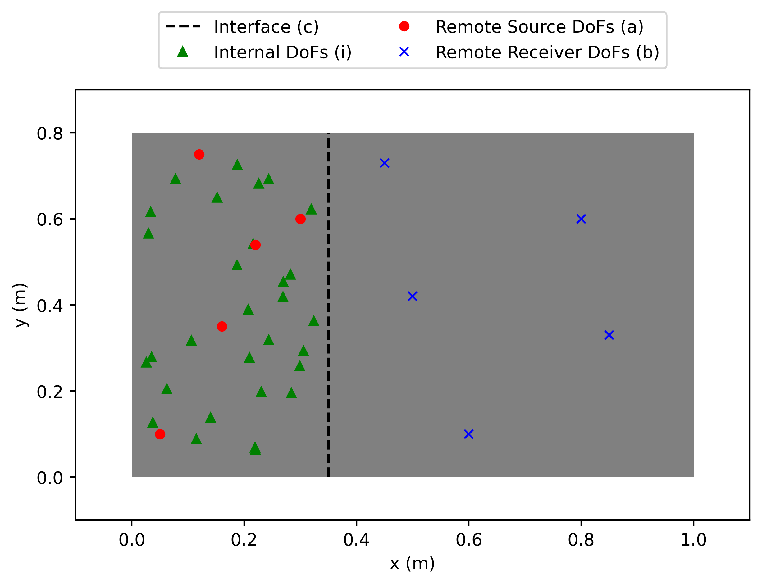
The continuous plate is divided into ‘source’ and ‘receiver’ subsystems by an imaginary interface, as illustrated in Figure 2. On the source side we define a set of remote observation DoFs \(a\) (red circles) and a set of internal excitation DoFs \(i\) (green triangles). On the receiver side we define a set of remote observation points \(b\) (blue crosses). Along the interface (dashed line) we define a set of point-like interface DoFs \(c\), which we vary in number to represent different levels of interface completeness.

The plate dimensions and material properties are: length \(L=1\) m, width \(W=0.8\) m, thickness \(H=0.005\) m, Young’s modulus \(E = 200\) GPa, density \(\rho = 7000\) and loss factor \(\nu=0.05\). We compute its FRFs using a modal summation approach including the out-of-plane \(z\) and \(x/y\) rotational DoFs. The number of interface points \(c\) is varied between 1 and 15 (i.e. 3 and 45 DoFs) to represent different levels of interface completeness.

import numpy as np
import matplotlib.pyplot as plt
from matplotlib.patches import Rectangle

def MAC(a,b):
    """
    Compute MAC similatiry criterion between complex vectors a and b

    Parameters
    ----------
    a : np.array, 1 or 2D (2nd dimension should be frequency)
        Complex vector.
    b : np.array, 1 or 2D (2nd dimension should be frequency)
        Complex vector.

    Returns
    -------
    MAC_out : np.array, 1D
        MAC similartity (0<MAC<1).

    """
    if len(a.shape) == 1:
        MAC_out = np.abs(np.inner(a,np.conj(b)))**2/(np.abs(np.inner(a,np.conj(a)))*np.abs(np.inner(b,np.conj(b))))
    elif len(a.shape) == 2:
        MAC_out = np.zeros(a.shape[1],dtype = float)
        for fi in range(a.shape[1]):
            MAC_out[fi] = np.abs(np.inner(a[:,fi],np.conj(b[:,fi])))**2/(np.abs(np.inner(a[:,fi],np.conj(a[:,fi])))*np.abs(np.inner(b[:,fi],np.conj(b[:,fi]))))

    return MAC_out

def simpSupPlateMS(dim, matProp, pos, freq, numM=30):
    """
    simpSupPlateMS models a simply supported plate using modal summation with
    sin-sin basis functions

    Parameters
    ----------
    dim : 3x1 numpy array
        Dimensions of plate: length x, length y, thickness - [lx, ly, h].
    matProp : 3x1 numpy array
        Material properties: density, Young's modulus, loss factor - [rho, E,
        nu].
    pos : Nx2 numpy array
        Simulation coordinates - [[x1, x2, ..., xN], [y1, y2, ..., yN]].
    freq : Mx1 numpy array
        Frequency vector - [f1, f2, ... fM].
    nM : Int, optional
        Highest modal order used in calculation. The default is 60.

    Returns
    -------
    Y : 3Nx3NxM numpy array
       Mobility matrix (including translational and rotational DoFs) at
       specified simulation positions. Translational and x/y rotational
       entries are grouped together for each coordinate.

    """

    m = dim[0]*dim[1]*dim[2]*matProp[0]  # Total mass of plate
    mI = dim[2]/np.sqrt(12)  # Moment of inertia
    G = matProp[1]/(3*(1-2*0.3))  # Longitudinal stiffness (mu = 0.3)
    cl = np.sqrt(G/matProp[0])  # Longitudual wave speed
    npts = np.size(pos, 1)  # Number of measurement points
    ndof = 3  # Number of DoFs at each measurement point
    nModes = numM**2  # Number of modes used in summation

    # Calculate natural frequencies and mode shapes
    wn = np.zeros(nModes, dtype=complex)  # Vector of radian frequencies
    r = np.zeros([ndof*npts, nModes], dtype=complex)  # Mode shape matrix
    ind = 0  # Mode index
    for n in range(1, int(np.sqrt(nModes))):
        for m in range(1, int(np.sqrt(nModes))):
            # Natural frequency
            wn[ind] = cl*mI*(np.pi**2)*((m/dim[0])**2 + (n/dim[1])**2)
            # Translational mode shape
            r[0:ndof*npts:3, ind] = 2*np.sin(np.pi*m*pos[0, :]/dim[0]) * \
                np.sin(np.pi*n*pos[1, :]/dim[1])
            # Rotational (x) mode shape
            r[1:ndof*npts:3, ind] = -2*(np.pi*m/dim[0]) * \
                np.cos(np.pi*m*pos[0, :]/dim[0]) * \
                np.sin(np.pi*n*pos[1, :]/dim[1])
            # Rotational (y) mode shape
            r[2:ndof*npts:3, ind] = 2*np.sin(np.pi*m*pos[0, :]/dim[0]) * \
                (np.pi*n/dim[1])*np.cos(np.pi*n*pos[1, :]/dim[1])
            ind = ind + 1
    wn2 = (1+1j*matProp[2])*wn**2  # Add structural damping

    # Calculate mobility matrix
    Yout = np.zeros([npts*ndof, npts*ndof, freq.shape[0]], dtype=complex)
    for fi in range(freq.shape[0]):
        w = 2*np.pi*freq[fi]
        W2 = np.ones([nModes, ], dtype=complex)*w**2
        D = wn2 - W2  # Calculate denominator
        Yout[:, :, fi] = (1j*w/m)*r@np.diag(1/D)@r.T

    return Yout

# %% Material properties
E = 200E9  # Young's modulus
rho = 7000  # Density
nu = 0.05  # Loss factor
nf = 1000
freq = np.logspace(np.log10(100), np.log10(5000), nf)  # Frequency array
# %% Set-up plate geometery
lx = 1  # Plate length
ly = 0.8  # Plate width
lz = 0.005  # Plate depth
cx = 0.35  # A-B interface (x-distance)
rng = np.random.default_rng(0)
n_rand = 30
xi = 0.025 + rng.random(n_rand) * (cx-0.05)
yi = 0.025 + rng.random(n_rand) * (ly-0.05)
# xi = np.array([0.035, 0.15, 0.26, 0.17, 0.23])  # A measurement points (x)
# yi = np.array([0.53, 0.65, 0.25, 0.04, 0.77])  # A measurement points (y)
ni = xi.shape[0]  # Number of interface points
xa = np.array([0.05, 0.12, 0.16, 0.22, 0.3])  # A measurement points (x)
na = xa.shape[0]  # Number of A points
ya = np.array([0.1, 0.75, 0.35, 0.54, 0.6])  # A measurement points (y)
xb = np.array([0.5, 0.6, 0.85, 0.8, 0.45])  # B measurement points (x)
nb = xb.shape[0]  # Number of B points
yb = np.array([0.42, 0.1, 0.33, 0.6, 0.73])  # B measurement points (y)

fig = plt.figure(figsize=(7, 4.5))
plt.xlim(-0.1, 1.1)
plt.ylim(-0.1, 0.9)
currentAxis = plt.gca()
currentAxis.add_patch(Rectangle((0, 0), lx, ly, facecolor="grey"))
plt.plot([cx, cx], [0, ly], color="black", linestyle='dashed', label='Interface (c)')
plt.plot(xi, yi, color='g', linestyle='None', marker="^", markersize=5.0, label='Internal DoFs (i)')
plt.plot(xa, ya, color='r', linestyle='None', marker="o", markersize=5.0, label='Remote Source DoFs (a)')
plt.plot(xb, yb, color='b', linestyle='None', marker="x", markersize=5.0, label='Remote Receiver DoFs (b)')
plt.xlabel('x (m)')
plt.ylabel('y (m)')
plt.legend(ncol = 2, loc='upper center', bbox_to_anchor=(0.5, 1.2))
plt.savefig('Figures/numsimdiag.png', dpi=400, bbox_inches='tight')
plt.close()

Figure 2: Layout of numerical plate example. Green triangles are internal excitation DoFs \(i\) and remote source DoFs \(a\). Blue crosses are remote receiver DoFs \(b\). The dashed line indicates the interface location \(c\), along which different numbers of interface DoFs are defined to represent different levels of interface completeness.

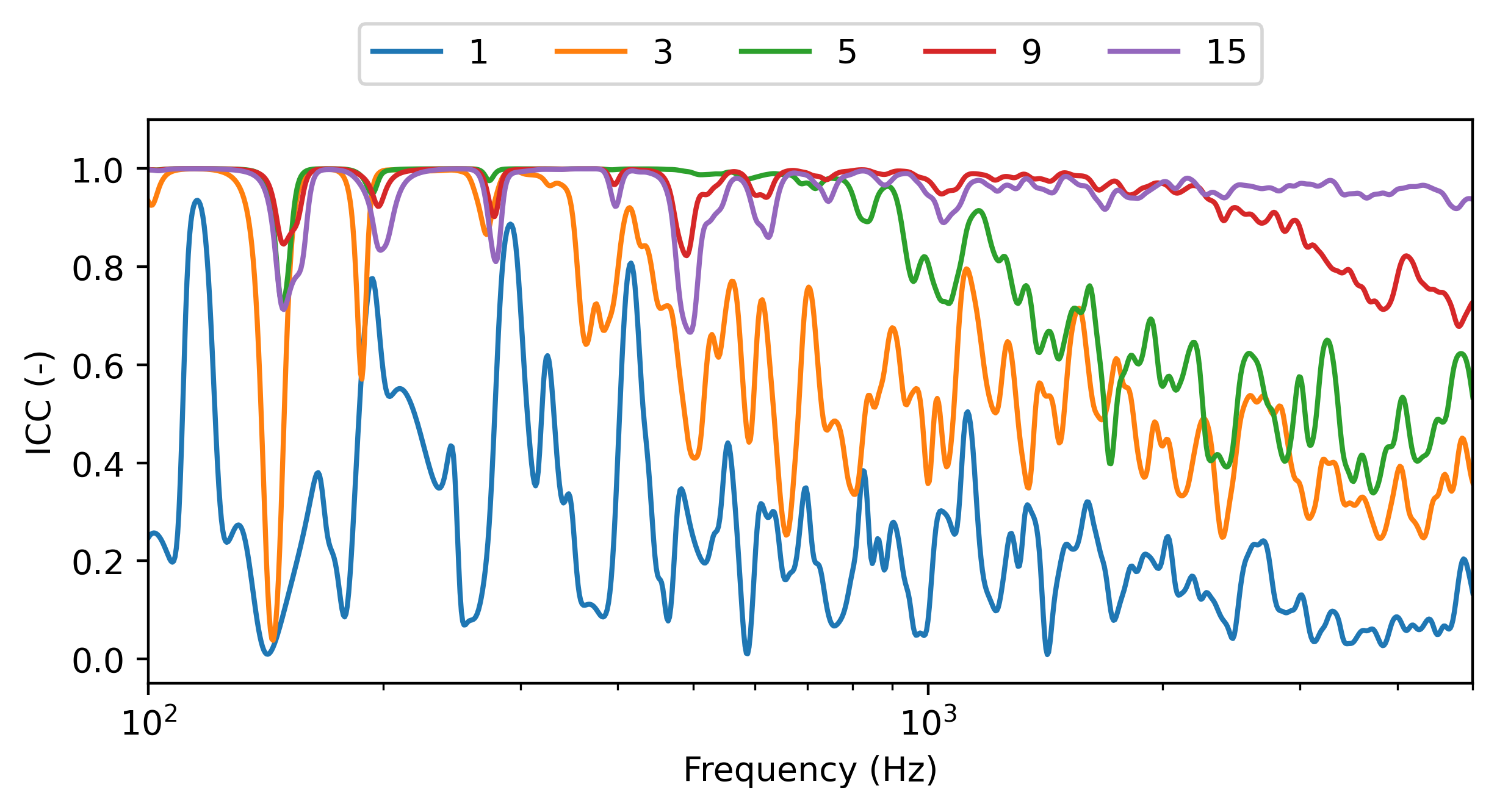
Using the remote source (\(a\)), interface (\(c\)), and remote receiver (\(b\)) DoFs defined above, we compute the FRF matrix of the full plate system and from this extract the direct transfer FRF matrix \(\mathbf{Y}_{Cba}\), alongside \(\mathbf{Y}_{Cbc_i}\), \(\mathbf{Y}_{Cc_ic_i}\) and \(\mathbf{Y}_{Cc_ia}\) which are used to reconstruct \(\mathbf{Y}_{Cba}^{(c_i)}\) and compute the ICC. The result for different levels of interface discretisation (i.e. different numbers of interface points) is shown in Figure 3. As expected, we see that as the number of interface DoFs increases, the ICC approaches 1, indicating a more complete interface representation.

# %% Compute direct and round trip FRF matrices and ICCs for different
# levels of interface completeness
ind = 0  # Initialize index
nCond = 5  # Number of interface conditions
nC = np.array([1, 3, 5, 9, 15])  # Number of interface DoFs (z, x/y rot)
ICC_mac = np.zeros((nCond, freq.shape[0]), dtype=float)  # Initialise
TICC = np.zeros((nCond, freq.shape[0]), dtype=float)
Tba_ex0 = np.zeros((freq.shape[0]), dtype=complex)
Tba_ex = np.zeros((nCond, freq.shape[0]), dtype=complex)
for nc in nC:  # Compute ICC including tran z and x/y rot for different # DoFs
    xc = np.ones(nc)*cx  # x coordinates of interface points
    yc = np.linspace(1, nc, nc)*ly/(nc+1)  # y coordinates of interface points
    x = np.hstack((xi, xa, xb, xc))  # Combine all x coordinates
    y = np.hstack((yi, ya, yb, yc))  # Combine all y coordinates
    xy = np.vstack((x, y))  # Form xy position array
    Y = simpSupPlateMS([lx, ly, lz],
                           [rho, E, nu], xy,
                           freq, numM=30)  # Compute full FRF matrix
    Yba = Y[3*ni+3*na:3*ni+3*na+3*nb, 3*ni:3*ni+3*na, :]  # Direct transfer FRF
    YbaRT = np.zeros(Yba.shape, dtype=complex)  # Allocate space
    na_ = 3
    Tba = np.zeros((3*nb, na_, nf), dtype=complex)  # Allocate space
    Tba_ = np.zeros((3*nb, na_, nf), dtype=complex)  # Allocate space
    for fi in range(freq.shape[0]):  # Loop over frequency
        Ybc = Y[3*ni+3*na:3*ni+3*na+3*nb, 3*ni+3*na+3*nb:, fi]
        Ycc = Y[3*ni+3*na+3*nb:, 3*ni+3*na+3*nb:, fi]
        Yca = Y[3*ni+3*na+3*nb:, 3*ni:3*ni+3*na, fi]
        YbaRT[:, :, fi] = Ybc @ np.linalg.pinv(Ycc) @ Yca

        Yai = Y[3*ni:3*ni+3*na, :3*ni,  fi]
        Ybi = Y[3*ni+3*na:3*ni+3*na+3*nb, :3*ni,  fi]
        Yci = Y[3*ni+3*na+3*nb:, :3*ni,  fi]

        T = Ybi @ np.linalg.pinv(np.vstack((Yai[0:na_,:],Yci)))  # Transmissibility matrix - constrained at interface
        Tba[:,:,fi] = T[:, :na_]  # Sub-transmissibility a->b

        Tba_[:,:,fi] = Ybi @ np.linalg.pinv(Yai[0:na_,:])  # Transmissibility matrix - unconstrained

    # TICC[ind,:] = np.mean(np.abs(Tba),axis=(0, 1))  # Compute TICC
    # TICC[ind,:] = np.linalg.norm(Tba, axis=(0, 1), ord='fro')
    Tba_ex[ind,:] = Tba[0,0,:]

    Tba_ex0[:] = Tba_[0,0,:]

    TICC[ind,:] = 1 - 2 * np.linalg.norm(Tba, axis=(0, 1),ord='fro')**2 / (np.linalg.norm(Tba, axis=(0, 1),ord='fro')**2 + np.linalg.norm(Tba_, axis=(0, 1), ord='fro')**2)

    ICC_mac[ind, :] = MAC(np.concatenate(Yba),
                          np.concatenate(YbaRT))  # Compute correlation ICC
    ind = ind + 1

fig, ax = plt.subplots(1, 1, figsize=(7, 3))
plt.semilogx(freq, ICC_mac[0, :], label='1')
plt.semilogx(freq, ICC_mac[1, :], label='3')
plt.semilogx(freq, ICC_mac[2, :], label='5')
plt.semilogx(freq, ICC_mac[3, :], label='9')
plt.semilogx(freq, ICC_mac[4, :], label='15')
plt.xlim((100, 5000))
plt.ylim((-0.05, 1.1))
plt.legend(ncol = 5, loc='upper center', bbox_to_anchor=(0.5, 1.2))
plt.xlabel('Frequency (Hz)')
plt.ylabel('ICC (-)')
plt.savefig('Figures/numsimicc.png', dpi=400, bbox_inches='tight')
plt.close()

Figure 3: Results of ICC for different levels of interface discretisation

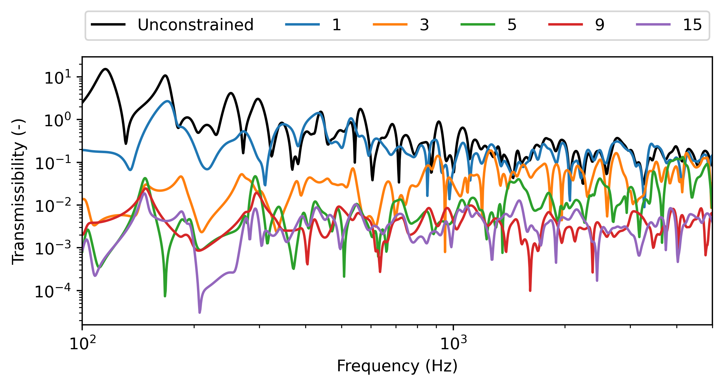
To avoid measuring a full set of FRFs, particularly the interface FRF matrix \(\mathbf{Y}_{Ccc}\), the TICC instead relies on the blocking constraints present in the definition of GT when computed using the response measurements at the interface. This blocking effect can be seen by examining the change in a transmissibility between \(a\) and \(b\) as a different number of interface DoFs are included in \(c\), as illustrated in Figure 4. We see a general descrease in the transmissibility magnitude as more interface DoFs are included, indicating the blocking of transmission paths across the interface.

fig, ax = plt.subplots(1, 1, figsize=(7, 3))
plt.loglog(freq, np.abs(Tba_ex0[:]),'k', label='Unconstrained')
plt.loglog(freq, np.abs(Tba_ex[0, :]), label='1')
plt.loglog(freq, np.abs(Tba_ex[1, :]), label='3')
plt.loglog(freq, np.abs(Tba_ex[2, :]), label='5')
plt.loglog(freq, np.abs(Tba_ex[3, :]), label='9')
plt.loglog(freq, np.abs(Tba_ex[4, :]), label='15')
plt.xlim((100, 5000))
# plt.ylim((-0.05, 1.1))
plt.legend(ncol = 6, loc='upper center', bbox_to_anchor=(0.5, 1.2))
plt.xlabel('Frequency (Hz)')
plt.ylabel('Transmissibility (-)')
plt.savefig('Figures/numsimtran.png', dpi=400, bbox_inches='tight')
plt.close()

Figure 4: Example transmissibilities obtained from different levels of interface discretisation

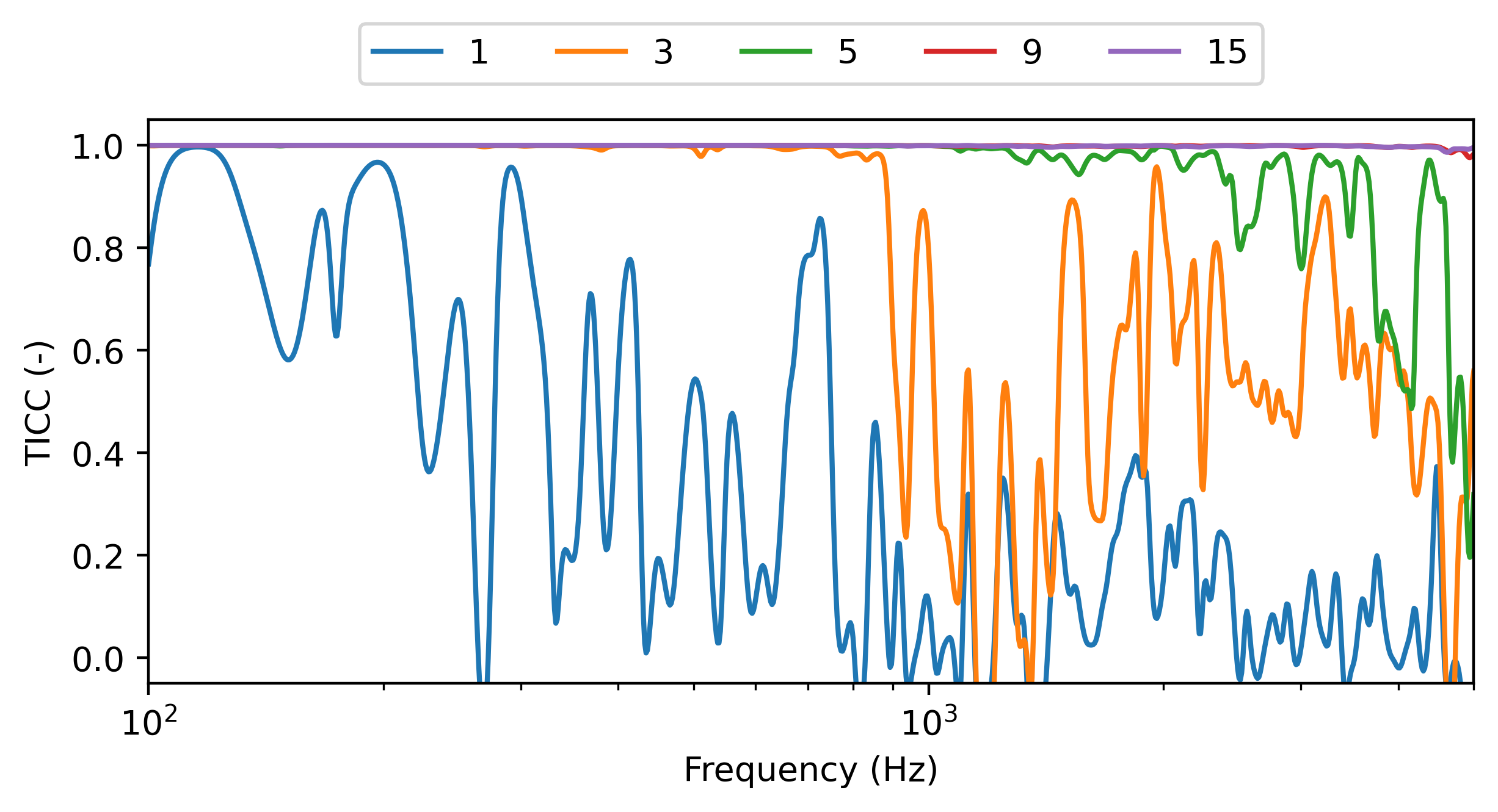
The blocking effect is more apparent when considering the TICC metric, as shown in Figure 5. As with the ICC, we see that as the level of interface discretisation is increased, the TICC tends to a value of 1, indicating a complete interface. It should be noted that whilst the ICC and TICC follow the same general trend, they quantify completeness in different ways, and are therefore not expected to give identical results.

fig, ax = plt.subplots(1, 1, figsize=(7, 3))
plt.semilogx(freq, TICC[0, :], label='1')
plt.semilogx(freq, TICC[1, :], label='3')
plt.semilogx(freq, TICC[2, :], label='5')
plt.semilogx(freq, TICC[3, :], label='9')
plt.semilogx(freq, TICC[4, :], label='15')
plt.xlim((100, 5000))
plt.ylim((-0.05, 1.05))
plt.legend(ncol = 5, loc='upper center', bbox_to_anchor=(0.5, 1.2))
plt.xlabel('Frequency (Hz)')
plt.ylabel('TICC (-)')
plt.savefig('Figures/numsimticc.png', dpi=400, bbox_inches='tight')
plt.close()

Figure 5: Results of TICC for different levels of interface discretisation

4 Experimental example - coupled beam-plate system

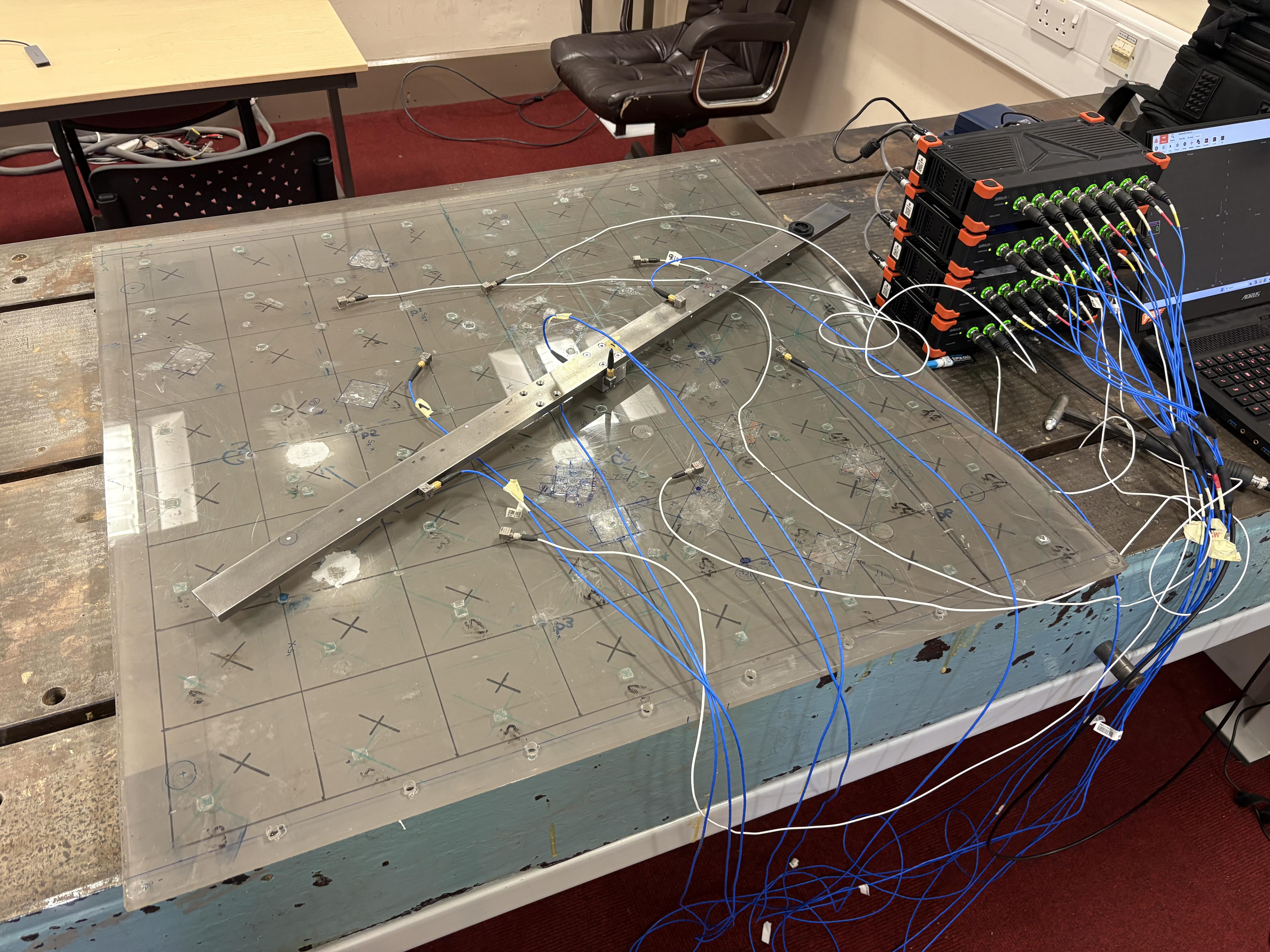
In this section we compare the ICC and TICC on a simple experimental case study. The assembly under study is shown in Figure 6 and comprises a steel beam rigidly coupled to a perspex plate at a single connection point.

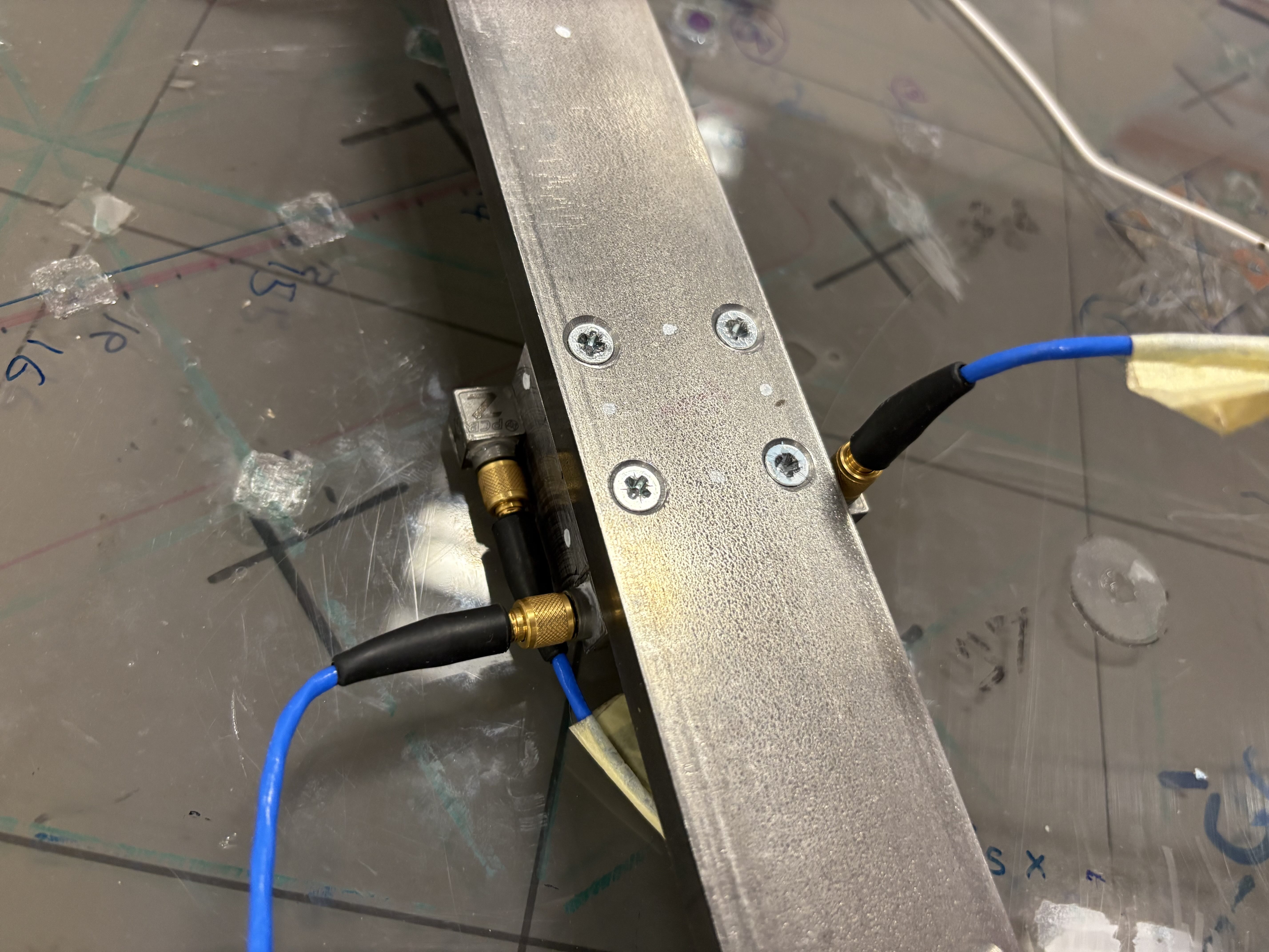
The interface connection is instrumented by three triaxial accelerometers and excited by 9 forces. A standard Virtual Point (VP) transformation is used to obtain a set of co-located interface DoFs at \(c\) in the translational \(x\), \(y\) and \(z\) directions and corresponding rotations \(\alpha\), \(\beta\) and \(\gamma\). To the plate we attatch two triaxial and 5 uniaxial accelerometers acting as our \(b\) DoFs for both ICC and TICC. Two further triaxials are fixed to the beam; for the TICC these act as the source-side \(a\) DoFs. In addition to the interface excitations, we excite the beam at 16 different locations; for the TICC these act as a set of ‘internal’ forces used to generate independent response vectors at \(a\), \(b\) and \(c\). For the ICC, these excitations instead act as the \(a\) DoFs (the source-side triaxials are not used). It should be noted that the excitations are purposefully performed in \(x\), \(y\) and \(z\) direction so to fully excite the interface. As such we would expect that to acheive a complete interface representation, all interface DoFs should be necessary.

(a) Wide shot.

(b) Interface close up.

Figure 6: Photo of experimental assembly used to compare the ICC and TICC.

Using the collected FRF data we compute the ICC and TICC for three different interface representations, including: all DoFs, translational-only DoFs (\(x\), \(y\), \(z\)), and translational+rotational DoFs (\(z\), \(\alpha\), and \(\beta\)).

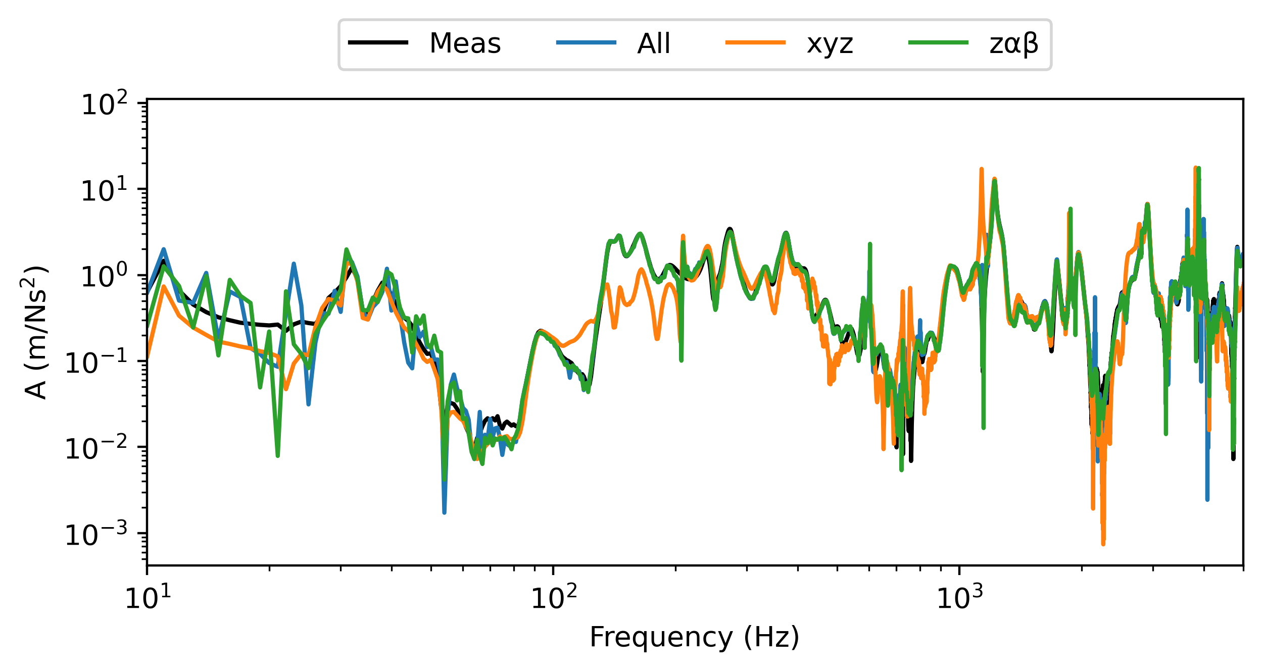
To compute the ICC we first reconstruct the FRF \(\mathbf{Y}_{Cba}^{(c_i)} = \mathbf{Y}_{Cbc_i}\mathbf{Y}_{Cc_ic_i}^{-1}\mathbf{Y}_{Cc_ia}\), which for a complete interface should yield exactly the transfer FRF \(\mathbf{Y}_{Cba}\). Shown in Figure 7 is an example of this reconstruction for each of the considered interface representations. We see that for the particular excitation and response positions chosen, all DoFs yields an FRF in close visual agreement with the direct measurement. Also in close agreement is that obtained when using tran+rot DoFs. In contrast, using the tran-only representation we see some notable deviations in the mid-high frequencies. At low frequencies however, we see that the tran-only DoFs do reasonably well, yielding an FRF with significantly less noise; this is on account of omitting the rotational DoFs which are known to have a greater sensitity to noise.

import scipy as sp
import scipy.io as sio
import numpy as np
import matplotlib.pyplot as plt


def MAC(a,b):
    """
    Compute MAC similatiry criterion between complex vectors a and b

    Parameters
    ----------
    a : np.array, 1 or 2D (2nd dimension should be frequency)
        Complex vector.
    b : np.array, 1 or 2D (2nd dimension should be frequency)
        Complex vector.

    Returns
    -------
    MAC_out : np.array, 1D
        MAC similartity (0<MAC<1).

    """
    if len(a.shape) == 1:
        MAC_out = np.abs(np.inner(a,np.conj(b)))**2/(np.abs(np.inner(a,np.conj(a)))*np.abs(np.inner(b,np.conj(b))))
    elif len(a.shape) == 2:
        MAC_out = np.zeros(a.shape[1],dtype = float)
        for fi in range(a.shape[1]):
            MAC_out[fi] = np.abs(np.inner(a[:,fi],np.conj(b[:,fi])))**2/(np.abs(np.inner(a[:,fi],np.conj(a[:,fi])))*np.abs(np.inner(b[:,fi],np.conj(b[:,fi]))))

    return MAC_out

def VP(fPos, sPos, fe, se, vpPos):
    """ Implement Virtual Point transformation for single connection

    Args:
        H (3D np.array (M x N x f), dtype=complex):
            FRF matrix
        fPos (2D np.array (N x 3), dtype=real):
            x, y, z coordinates of force positions
        sPos (2D np.array (M x 3), dtype=real):
            x, y, z coordinates of sensor positions
        fe (2D np.array (N x 3), dtype=real):
            ex, ey, ez orientation of applied forces
        se (2D np.array (M x 3), dtype=real):
            ex, ey, ez orientation of sensors
        vpPos (1D np.array (3 x 1), dtype=real):
            x, y, z position of virtual points
    """
    fRPos = fPos-vpPos  # Force position relative to VP
    sRPos = sPos-vpPos  # Sensor position relative to VP
    Rs = np.zeros((sPos.shape[0], 6))
    for si in range(sPos.shape[0]):
        # Build transformation matrix for each response point
        Rsi = np.array([[1, 0, 0, 0, sRPos[si, 2], -sRPos[si, 1]],
                        [0, 1, 0, -sRPos[si, 2], 0, sRPos[si, 0]],
                        [0, 0, 1, sRPos[si, 1], -sRPos[si, 0], 0]])
        # Sensor displacement due to Virtual Point displacement
        # (1x6 vector for each sensor):
        Rs[si, :] = se[si, :]@Rsi
    Ts = np.linalg.pinv(Rs)
    Rf = np.zeros((fPos.shape[0], 6))
    for fi in range(fPos.shape[0]):
        # Build transformation matrix for each response point
        Rfi = np.array([[1, 0, 0, 0, fRPos[fi, 2], -fRPos[fi, 1]],
                        [0, 1, 0, -fRPos[fi, 2], 0, fRPos[fi, 0]],
                        [0, 0, 1, fRPos[fi, 1], -fRPos[fi, 0], 0]])
        # Sensor displacement due to Virtual Point displacement
        # (1x6 vector for each sensor):
        Rf[fi, :] = Rfi.T@fe[fi, :].T
        Tf = np.linalg.pinv(Rf)
    return Ts, Tf, Rs, Rf

# Load data
nf = 27
nr = 26
temp = sio.loadmat('Data/Test1/f1.mat')
f = temp["Data1_X_MT_FRF_H1_10Xplus_29Zplus_Imag"]
H = np.zeros((f.shape[0], nr, nf), dtype=complex)
COH = np.zeros((f.shape[0], nr, nf), dtype=complex)
for i in range(1,nf):
    temp = sio.loadmat('Data/Test1/f' + str(i) + '.mat')
    for j in range(1,nr):
        H[:,j-1,i-1] = (temp['Data1_MT_FRF_H1_' + str(j) + 'Xplus_29Zplus_Real'] + 1j*temp['Data1_MT_FRF_H1_' + str(j) +'Xplus_29Zplus_Imag']).squeeze()
        COH[:,j-1,i-1] = (temp['Data1_MT_Coherence_' + str(j) + 'Xplus_29Zplus'] + 1j*temp['Data1_MT_Coherence_' + str(j) +'Xplus_29Zplus']).squeeze()

# Built TMs
E1 = np.array([[0, 0, -1],[1, 0, 0],[0, -1, 0]])
E2 = np.array([[0, -1, 0],[0, 0, 1],[-1, 0, 0]])
E3 = np.array([[1, 0, 0],[0, 1, 0],[0, 0, 1]])
R1 = np.array([-15, -25, 20])*1e-3
R2 = np.array([-25, 15, 20])*1e-3
R3 = np.array([15, 25, 5])*1e-3
sPos = np.stack((R1,R1,R1,R2,R2,R2,R3,R3,R3))
se = np.vstack((E1,E2,E3))

e1 = np.array([0,0,-1])
e2 = np.array([0,0,-1])
e3 = np.array([0,0,-1])
e4 = np.array([0,0,-1])
e5 = np.array([0,1, 0])
e6 = np.array([0,-1,0])
e7 = np.array([0,-1,0])
e8 = np.array([-1,0,0])
e9 = np.array([-1,0,0])
r1 = np.array([-15, 0, 35])*1e-3
r2 = np.array([0, 15, 35])*1e-3
r3 = np.array([15, 0, 35])*1e-3
r4 = np.array([0, -15, 35])*1e-3
r5 = np.array([15, -20, 20])*1e-3
r6 = np.array([-15, 20, 20])*1e-3
r7 = np.array([15, 20, 20])*1e-3
r8 = np.array([20, 15, 25/2])*1e-3
r9 = np.array([20, -15, 25/2])*1e-3
fe = np.stack((e1,e2,e3,e4,e5,e6,e7,e8,e9))
fPos = np.stack((r1,r2,r3,r4,r5,r6,r7,r8,r9))

Ts_c, Tf_c, Rs, Rf = VP(fPos, sPos, fe, se, np.array([0,0,0]))

Tr = sp.linalg.block_diag(Ts_c,np.eye(6),np.eye(11))
Tf = sp.linalg.block_diag(Tf_c,np.eye(18))

Hvp = Tr@H@Tf.T

Yba_all = Hvp[:,12:,:6]@np.linalg.inv(Hvp[:,:6,:6])@Hvp[:,:6,6:]
Yba_xyz = Hvp[:,12:,:3]@np.linalg.inv(Hvp[:,:3,:3])@Hvp[:,:3,6:]
Yba_zαβ = Hvp[:,12:,2:5]@np.linalg.inv(Hvp[:,2:5,2:5])@Hvp[:,2:5,6:] 

ICC_all = np.zeros((f.shape[0]),dtype=complex)
ICC_xyz = np.zeros((f.shape[0]),dtype=complex)
ICC_zαβ = np.zeros((f.shape[0]),dtype=complex)
for i in range(f.shape[0]):
    ICC_all[i] = MAC(Hvp[i, 12:, 6:].flatten(), Yba_all[i,:,:].flatten())
    ICC_xyz[i] = MAC(Hvp[i, 12:, 6:].flatten(), Yba_xyz[i,:,:].flatten())
    ICC_zαβ[i] = MAC(Hvp[i, 12:, 6:].flatten(), Yba_zαβ[i,:,:].flatten())

Uc = Hvp[:,:6,6:]
Ua = Hvp[:,6:12,6:]
Ub = Hvp[:,12:,6:]
T = Ub @ np.linalg.pinv(np.concat((Ua,Uc),axis=1))  # Transmissibility matrix - constrained at interface
Tba = T[:, :, :6]  # Sub-transmissibility a->b
Tba_= Ub @ np.linalg.pinv(Ua)  #
TICC_all = 1 - 2 * np.linalg.norm(Tba, axis=(1, 2),ord='fro')**2 / (np.linalg.norm(Tba, axis=(1, 2),ord='fro')**2 + np.linalg.norm(Tba_, axis=(1, 2), ord='fro')**2)

Uc_xyz = Hvp[:,:3,6:]
T = Ub @ np.linalg.pinv(np.concat((Ua,Uc_xyz),axis=1))  # Transmissibility matrix - constrained at interface
Tba = T[:, :, :6]  # Sub-transmissibility a->b
Tba_= Ub @ np.linalg.pinv(Ua)  #
TICC_xyz = 1 - 2 * np.linalg.norm(Tba, axis=(1, 2),ord='fro')**2 / (np.linalg.norm(Tba, axis=(1, 2),ord='fro')**2 + np.linalg.norm(Tba_, axis=(1, 2), ord='fro')**2)

Uc_zαβ = Hvp[:,2:5,6:]
T = Ub @ np.linalg.pinv(np.concat((Ua,Uc_zαβ),axis=1))  # Transmissibility matrix - constrained at interface
Tba = T[:, :, :6]  # Sub-transmissibility a->b
Tba_= Ub @ np.linalg.pinv(Ua)  #
TICC_zαβ = 1 - 2 * np.linalg.norm(Tba, axis=(1, 2),ord='fro')**2 / (np.linalg.norm(Tba, axis=(1, 2),ord='fro')**2 + np.linalg.norm(Tba_, axis=(1, 2), ord='fro')**2)

n,m = 2,1
fig, ax = plt.subplots(1, 1, figsize=(7, 3))
plt.loglog(f, np.abs(Hvp[:, 12+n, 6+m]), 'k', label='Meas')
plt.loglog(f, np.abs(Yba_all[:, 0+n, 0+m]), label='All')
plt.loglog(f, np.abs(Yba_xyz[:, 0+n, 0+m]), label='xyz')
plt.loglog(f, np.abs(Yba_zαβ[:, 0+n, 0+m]), label='zαβ')

plt.xlim((10, 5000))
# plt.ylim((-0.05, 1.05))
plt.legend(ncol = 5, loc='upper center', bbox_to_anchor=(0.5, 1.2))
plt.xlabel('Frequency (Hz)')
plt.ylabel('A (m/Ns$^2$)')
plt.savefig('Figures/expobval.png', dpi=400, bbox_inches='tight')
plt.close()

Figure 7: Example FRF reconstructions (as used by the ICC) obtained using different levels of interface discretisation

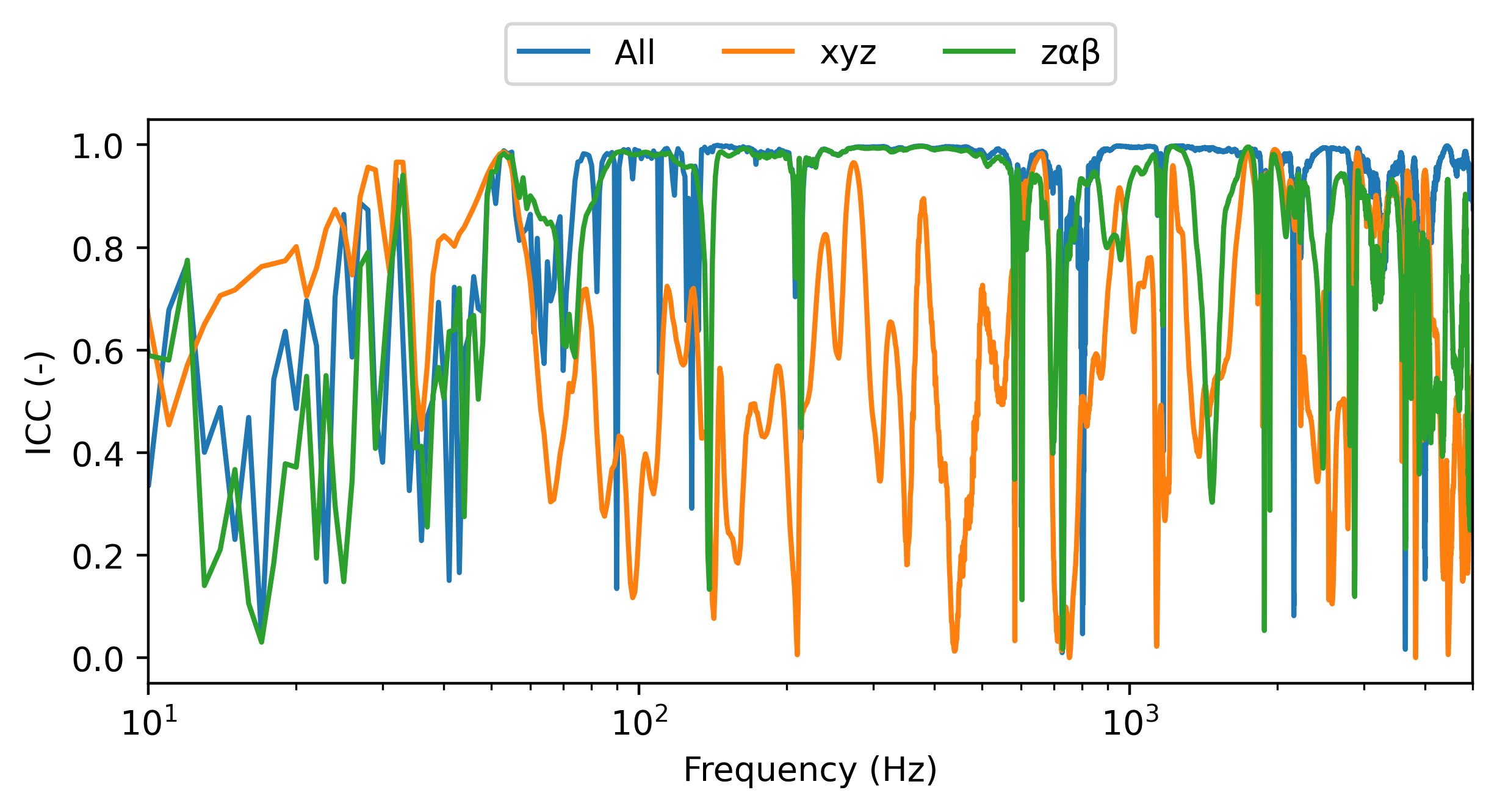
The results in Figure 7 show just one FRF of the \(11\times 16\) FRF matrix \(\mathbf{Y}_{Cba}^{(c_i)}\). The ICC provides a single value comparison of all reconstructed FRFs together. We plot the computed ICC for each interface representation in Figure 8. As expected, we see that in the mid-high frequency including all DoFs yields the highest level of completeness, followed by the tran+rot representation which drops off at higher frequencies. The tran-only DoFs perform poorly across the entire frequency range, though still perform best at low frequencies.

It should be noted that at low frequencies, the low ICC is not a result of incompleteness, rather the influence of noise on the measured FRFs.

fig, ax = plt.subplots(1, 1, figsize=(7, 3))
plt.semilogx(f, np.abs(ICC_all),label='All')
plt.semilogx(f, np.abs(ICC_xyz),label='xyz')
plt.semilogx(f, np.abs(ICC_zαβ),label='zαβ')
plt.xlim((10, 5000))
# plt.ylim((-0.05, 1.05))
plt.legend(ncol = 5, loc='upper center', bbox_to_anchor=(0.5, 1.2))
plt.xlabel('Frequency (Hz)')
plt.ylabel('ICC (-)')
plt.savefig('Figures/expICC.png', dpi=400, bbox_inches='tight')
plt.close()

Figure 8: ICC of experimental case study using different interface representatons: all DoFs, translaitonal xyz, and translational z with x/y rotations

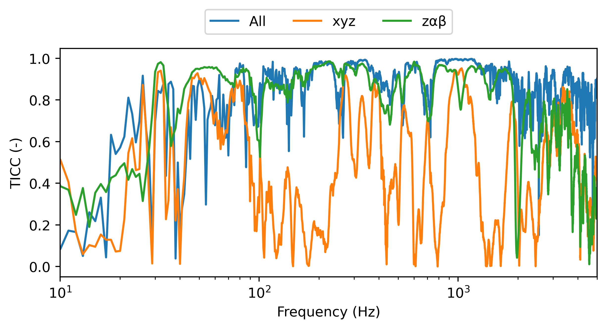
Shown in Figure 9 are the TICCs for each of the representations used above. Note that in this example, to enable fair comparison with the ICC, the TICCs are obtained using FRF-based measurements of the GT, as opposed to operational responses.

The results of the TICC largely follow the that of the ICC, as expected given that they are fundementally based on the same blocking constaints. Over the mid frequency range the all and tran+rot representations are in good agreement and indicate high level of completeness. At higher frequencies we see the tran+rot TICC begin to fall off, indicating an imporant contribution of the neglected in-plane/rotational \(z\) DoFs over this range. Like the ICC, the tran-only representation performs poorly over the entire frequency range. Overall, comparing Figure 8 and Figure 9 we see strong similarities between the two metrics.

fig, ax = plt.subplots(1, 1, figsize=(7, 3))
plt.semilogx(f, np.abs(TICC_all),label='All')
plt.semilogx(f, np.abs(TICC_xyz),label='xyz')
plt.semilogx(f, np.abs(TICC_zαβ),label='zαβ')
plt.xlim((10, 5000))
# plt.ylim((-0.05, 1.05))
plt.legend(ncol = 5, loc='upper center', bbox_to_anchor=(0.5, 1.2))
plt.xlabel('Frequency (Hz)')
plt.ylabel('TICC (-)')
plt.savefig('Figures/expTICC.png', dpi=400, bbox_inches='tight')
plt.close()

Figure 9: TICC of experimental case study using different interface representatons: all DoFs, translaitonal xyz, and translational z with x/y rotations

From an experimental perspective we beleive that of the two metrics the TICC is the more robust, as it relies on only a single set of source-side excitations, which can be either artifical or operational in nature. In contrast, the ICC requires excitations both remotely on the source and around the connecting interface. These latter excitations are often difficult to perform on real engineering sturcutres due to limited access to the interface, and so can introduce significant errors. Recalling that the interface FRF \(\mathbf{Y}_{Ccc}\) must be inverted for the ICC these interface excitations are also the most important to get right as any errors are amplified by the inversion process. As such, it can be quite time consuming to obtain relibale interface excitations.

For the TICC, the only additional requirement over the ICC is the attachement of some reponse sensors on the source; this is the cost of avoiding interface excitations.

5 Conclusions

In this paper we have proposed a generalised transmissibility-based interface completeness criterion termed the TICC.

Whilst the ICC and TICC share the same purpose–to quantify the level of interface completeness–they do so in different ways and so should be interpreted differently. The ICC describes how well a set of artifical blocked forces, obtained over the interface \(c\), can reproduce the response within the recevier, which is measured directly and used as a comparison. The TICC instead considers the (normalised) signal level within the receiver before and after the measured interface DoFs are constrained, with the understanding that for a complete interface the signal level should be 0.

We compare the ICC and TICC on a pair of numerical and experimental examples. In both cases the TICC follows the same general trend as the ICC; as the number of interface DoFs increases both metrics tend towards 1. The advantages of the TICC are that 1) it can be obtained with output-only response measurements, FRFs or a combination thereof, and 2) if FRFs are used, no exctiations are required at the interface. The TICC appears to offer a most robust quantification of interface completeness, with reduced experimental effort over the ICC.

The experimental example considered in this paper is a relatively simple one. Further verification of the TICC is required on more complex assemblies, in particular using output-only and mixed operational states.

References

[1]

J. Meggitt and A. Moorhouse, Experimental vibro-acoustics: In situ and blocked force methods for component-based simulation and virtual prototyping. CRC Press, 2025.

[2]

J. Meggitt and A. Moorhouse, “On the completeness of interface descriptions and the consistency of blocked forces obtained in situ,” Mechanical Systems and Signal Processing, vol. 145, p. 106850, 2020.

[3]

H. acoustics, “HEAD acoustics ArtemiS SUITE 17. Analyze more efficiently, develop smarter.” [https://www.example.com](https://www.head-acoustics.com/news-events/press-releases/press-details/show/head-acoustics-artemis-suite-17-analyze-more-efficiently-develop-smarter/), 2026. Available: [(https://www.head-acoustics.com/news-events/press-releases/press-details/show/head-acoustics-artemis-suite-17-analyze-more-efficiently-develop-smarter/)]

[4]

N. Maia, A. Urgueira, and R. Almeida, “Whys and wherefores of transmissibility,” Vibration Analysis and Control: New Trends and Developments, p. 197, 2011.

[5]

A. Moorhouse, A. Elliott, and T. Evans, “In situ measurement of the blocked force of structure-borne sound sources,” Journal of sound and vibration, vol. 325, no. 4–5, pp. 679–685, 2009.

[6]

K. Wienen, M. Sturm, A. Moorhouse, and J. Meggitt, “Generalised round-trip identity—for the determination of structural dynamic properties at locations inaccessible or too distant for direct measurement,” Journal of Sound and Vibration, vol. 511, p. 116325, 2021.

[7]

R. J. Allemang, “The modal assurance criterion–twenty years of use and abuse,” Sound and vibration, vol. 37, no. 8, pp. 14–23, 2003.

[8]

M. Haeussler, T. Mueller, E. Pasma, J. Freund, O. Westphal, and T. Voehringer, “Component TPA: Benefit of including rotational degrees of freedom and over-determination,” in Proceedings of the international conference on noise and vibration engineering, leuven, belgium, 2020, pp. 7–9.

[9]

M. Wegerhoff, R. Sottek, and H. Brücher, “A bridging technology to combine test and simulation with in-situ TPA,” SAE Technical Paper, 2020.